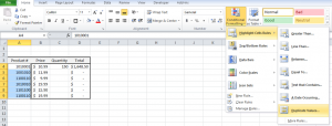
When inputting lists into Excel there is often a need to have a unique instance of every list item. For example item numbers or product names are very important to avoid confusion. Sequential serial numbers can be done with a formula but logical numbers (first digit denotes product category, second digit is subcategory, third and fourth are unique item) and manually assigned names are more difficult to auto generate. Excel has a built in function to find duplicate values, and even remove them.
 |
| Select Duplicate Value from the Conditional Formatting Toolbar |
The first step is to find duplicates. This can be done through a Conditional Formatting rule. Select the relevant cells (columns or rows are available selections) then select “Highlight Cell Rules” and “Duplicate Values” from the Home tab on the toolbar.
 |
| Choose how to format duplicate cells |
This brings up a dialog box on how to format. Changing the fill color makes it easy to see duplicates. Note that this does not count the number or duplicates but instead simply highlights any value that appears more than once.
